LASSO and RIDGE Linear regressions & L1 and L2 regularizations - the impact of the penalty term

	Teaching (Today for) Tomorrow: Bridging the Gap between the Classroom and Reality 3rd International Scientific and Art Conference Faculty of Teacher Education, University of Zagreb in cooperation with the Croatian Academy of Sciences and Arts
Siniša Opić Faculty of Education, University of Zagreb, Croatia sinisa.opic@ufzg.hr

Section - Education for innovation and research

Paper number: 1

Category: Original scientific paper

Abstract

Lasso and Ridge regressions are useful enhancements to ordinary least squares (OLS) regression, utilizing L1 and L2 regularization techniques. The main idea behind these methods is to balance the simplicity of the model with its accuracy by adding a penalty term to the existing regression formula. This approach leads to a significant reduction in the regression coefficients, potentially reducing some to zero (in the case of L1 regularization). These enhancements improve accuracy, increase R², lower mean squared error (MSE), eliminate non-significant coefficients, address the issue of multicollinearity among predictors, and most importantly, help prevent overfitting. In the empirical section of the study, both L1 (LASSO) and L2 (RIDGE) regression analyses were conducted on a dataset comprising 156 samples. A cross-validation procedure was employed with λ values ranging from 1 to 20 (with λmax=20, λmin = 0.5, and λ intervals of 1), using 5 folds. The results indicated that the application of Ridge regression, when compared to OLS, led to a reduction in the Beta coefficient, an increase in R², and a decrease in the Mean Squared Error (MSE). Furthermore, no significant discrepancies were found between the R² values for the training and holdout datasets, suggesting that the model is robust. However, in comparison, L1 regularization (LASSO) was performed, and the values ​​of all betas for all categories of predictor variables are zero (βstd=0; B=0); β=0 which indicates the impossibility of interpreting the regression model (type 2 error). LASSO and RIDGE regressions are iterative procedures, and their results depend on randomization, the number of k-fold cross-validations and k-iterations, the percentage of training and testing data, and the value of lambda (although this is a minor problem), so you should be careful when using them.

Key words:

Lasso regression, L1, L2 regularization, MSE, overfitting, penalty term, Ridge regression,  The sum of squared residuals

Introduction to linear regression (OLS)

The purpose of linear regression analysis is to determine the best-fitting line that accurately reflects the data by minimizing the sum of squared residuals, using the ordinary least squares (OLS) method. This relationship is described by the regression equation Y = a + bx, which can also be expressed as Y = β₀ + β₁x. In this equation, Y represents the dependent variable, β₀ (or a) is the constant (intercept), β₁ (or b) is the slope, and x is the independent variable.

Similarly, when using multiple predictors (independent variables), the equation can be expressed as Y = β₀ + β₁x + β₂x + ... + β_nx. By applying this regression equation, we can calculate the estimated value of the dependent variable for each new value of the predictors.

The slope of the regression line indicates its predictive power; a steeper line suggests better predictions. The formula for calculating the slope (b) is: b=   On the regression line, we find the estimated values of the dependent variable, while the difference between the actual values (y) and the estimated values () along the line is called the residual, defined as:

 e = (y-). The purpose of defining the regression line is to minimize these residuals; thus, a smaller difference between the actual and estimated values is desirable.

In regression analysis involving two variables, the sums of squares provide a clear definition of their relationship. If the regression line perfectly fits the data points, the sum of squares would equal zero. Linear regression analysis examines the relationships between different sums of squares (SS):

·      SSR (sum of regression squares) = ∑ ()² This measures the squared differences between the estimated values and the mean of y, 

·      Total Sum of Squares  SST =  ∑ ()²   i.e. the squared sum of the differences between the observed value of the variable y and its arithmetic mean

·      and the Residual sum of squares SSE = ∑ (   which represents the squared differences between the observed and estimated values of y.

 

Lastly, we define the coefficient of determination (R²) as follows: Vrh obrascaR²=  This coefficient indicates the proportion of the total variability in the dependent variable that can be explained by the independent variables. An alternative expression for R²=   (compare Nelson, Biu & Onu, 2004).

Figure 1 shows this graphically (an example of a study on the relationship between hours of practice playing the piano and the number of mistakes in playing)

 

Dno obrasca

 

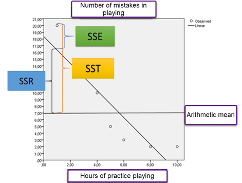
Figure 1  - sum of squares in OLS

From the values ​​of the regression parameters (R², R²_adjust, β...) we conclude about the validity and power of the predictive regression model. However, the values ​​of linear regression analysis (OLS) statistics are significantly affected by e.g. sample size, collinearity/multicollinearity, autocorrelation of residuals, linear dependence, outliers... From the above, LASSO and RIDGE linear regressions are a kind of control and upgrade of OLS linear regression (Marquardt & Snee, 1975; Hoerl, & Kennard, 1975, Irandoukht, 2021).

 

LASSO and RIDGE regressions

 

LASSO regression (Least Absolute Shrinkage and Selection Operator) is L1 regularization. The purpose of LASSO regression is to find a balance between the simplicity of the model and its accuracy by adding a penalty term to the existing regression model. Such an approach indicates a significant reduction of the regression coefficients, even down to the value of zero (0). Originally, LASSO regression was created in the field of geophysics, although it gained more popularity from the author Tibshirani (1996), who gave it its name.

 

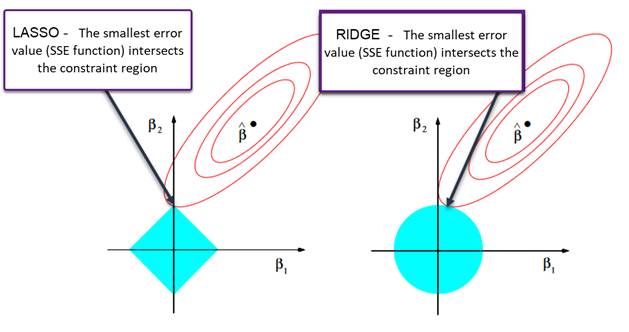
Figure 2 -SSE and regression constraints (adjusted according to Hastie, Tibshirani & Friedman, 2009).

 

Figure 2 shows the constraint region determined by the Ridge and Lasso regression. Due to the fact the Ridge regression constraints have no corners, solutions with zero beta coefficients are less likely than at Lasso (according to Kampe, Brody, Friesenhahn, Garret and Hegy, 2017).

 

RIDGE regression is a form of L2 regularization. The goal is to create a new regression line that does not fit the training data too perfectly, thereby introducing a certain level of bias as the line adjusts to the data. By increasing this bias, we can reduce the total variance. Using Ridge regression, we create a regression line that initially adapts less to the data, which can lead to improved predictions, especially in the case of small sample sizes.

The key aspect of this method is that we can have fewer respondents than variables, which is not the case with Ordinary Least Squares (OLS) regression. As the value of Lambda decreases, the slope of the regression line becomes steeper. When Lambda equals 0, the penalty for Ridge regression is zero, meaning the sum of squared residuals is minimally reduced; in this case, the regression line remains the same as the OLS line. As Lambda increases, the slope of the regression line decreases compared to the initial OLS line. In theory, a higher value of Lambda will result in a flatter regression line, and it is possible for the slope to reach 0.

The increasing slope of the lines suggests that the predictive model (Ordinary Least Squares, or OLS) is improving. However, a problem arises when making comparisons due to the growing influence of the x-axis values on the y-axis. When the regression line (OLS) is very steep, the estimated values for the y-axis become highly sensitive to even minor changes in the x-axis. To address this issue, cross-validation is employed to determine the optimal Lambda value that minimizes variance. RIDGE regression is used to divide the data into two groups: training data and testing data.  OLS is applied to the training data to generate a regression line. This regression line can be analyzed in terms of bias and variance concerning the testing data. A model with a lower bias in the training data typically exhibits greater variance in the testing data. The goal is to improve the relationship between the variables but on the principle of linear dependence. This discrepancy between the actual association relationship and the regression (in this case OLS) is biased.

By introducing a new RIDGE regression line that minimizes the sum of squared errors, a RIDGE regression penalty (lambda +slope²) is applied. This penalty reduces the influence of predictor variables on the dependent variable, which is particularly useful for identifying variables that have a smaller impact on the outcome. This approach helps control for these less significant variables. A common issue with ordinary least squares (OLS) regression is that adding more regressor variables can artificially inflate the coefficient of determination (R²), which represents the total variability of the dependent variable that can be explained by the predictor variables. In this case, it is about overfitting, i.e. too good agreement with existing data, but not so good when it comes to predicting new values ​​using the regression equation. This is especially important when it comes to multiple predictor variables and when they correlate because then multicollinearity is controlled using penalty values ​​(especially LASSO regression);  individual correlated variables are thrown out (because the regression coefficients decrease to 0 values), i.e. only individual variables from correlated groups of variables are singled out (beta coefficients are higher).  The biggest benefit of RIDGE regression (but also LASSO) is the influence (control) of multicollinearity that affects regression parameters (insight using VIF in OLS regression). Multicollinearity also affects the covariance matrix and can lead to an almost singular matrix. This is a problem because it can make the inverse matrix unstable. The solution lies in reducing the parameters, i.e. reduced eigenvalue, i.e. ensuring that the eigenvalues ​​in the covariance matrix are always positive, i.e. suitable for inversion (X′X + X′X + λI; I = inverse matrix). Although both RIDGE and LASSO regressions are part of linear models, they can also be used in non-parametric nonlinear regressions such as Logistic and Polynomial.

For a small value of λ, the variance of the RIDGE regression dominates the MSE, which is to be expected since the estimated λ of the RIDGE regression is close to the unbiased ML (maximum likelihood) regression estimate. For a larger value of λ, the variance decreases and the bias dominates the MSE (increases). Analogously, for very small values ​​of λ RIDGE regression, the increase in variance exceeds the increase in its own bias. (Wessel van Wieringen, 2023, Fig. 3a). Analogous to Figure 3b; MSE[ ˆβ(λ)] < MSE[ ˆβ(0)] for λ < 7 id est. by increasing lambda, the Ridge regression estimator outperforms its ML value.

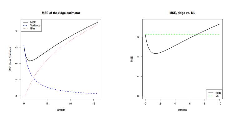
Figure 3a (left) - Relationship between MSE and bias, RIDGE regression variance
for different λ (after Weseel van Wieringen, 2023) 

Figure 3b (right) - MSE, RIDGE vs, ML

Regularization L1, L2

Regularization is a process that helps reduce overfitting and control the coefficients in statistical models. Walker (2004) compares Ordinary Least Squares (OLS) and RIDGE regression models using non-experimental data and highlights the superior accuracy of the RIDGE regression model (also Dempster, Schatzoff & Wermuth, 1977;  Kennedy, 1988). When deciding which method to use, the authors note that the choice depends on the context and the objectives of the research. However, regarding multicollinearity—which can lead to decreased validity and accuracy - OLS should definitely not be used. Instead, the RIDGE regression model is recommended.

L1 regularization, also known as Lasso regularization, is defined by the equation L₁ = λ (|β₁| + |β₂| + … + |βₚ|), where the penalty term is represented as  . In L1 regularization, as opposed to L2 regularization, the focus is on the absolute values of the coefficients (β). This is because the parameters in the loss function can have negative values, which indicates a decrease in the function's value. The solution provided by L1 regularization involves adding the absolute values of the parameters (β). This process tends to reduce the beta coefficients more significantly, leading to more reliable predictions.

L2 regularization, also known as Ridge regression, is very similar to L1 regulation, but with one key difference: in L2 regularization, the parameters (beta) are not treated as absolute values. Instead, the penalty term is expressed as L2 = λ (β₁ + β₂ + … + βₚ). Another approach that combines both L1 and L2 regularization is called Elastic Net. The efficiency of the cost function in both L1 and L2 regulation depends on the value of lambda. When lambda equals 0, the results are identical to those obtained from Ordinary Least Squares (OLS) regression, which highlights the need for larger lambda values. The optimal lambda value is the one that minimizes the Mean Squared Error (MSE) on the validation dataset. MSE is calculated as MSE = SSE/n, where SSE is the sum of squared errors, or MSE = which is analogous to the Loss or cost function. When working with cost functions, it is important to be cautious about their size. Introducing a penalty term can lead to an insignificant model by increasing the type 2 error. Cross-validation is one effective solution; it involves comparing subsets of data across multiple iterations (k iterations). The optimal lambda value is identified as the one that yields the smallest deviation between the testing and training data. If the coefficients derived from the training dataset yield accurate predictions for the test dataset, the lambda values can be kept low. However, if the coefficients result in poor predictions, the lambda values will need to be higher. Cross-validation helps to prevent overfitting across all datasets (according to Van del Velde, Piersoul, De Smet, and Rupper, 2021).

Empirical part

The matrix of a non-experimental research design (n=156) was used in which the role of 3 predictors (father's education, non-violent behavior and type of school) on the general success of students was tested. Regression analysis determined the total variability of general school success, which can be explained by the role of predictors, R²=0.226, R²_adjust=0.211.

ANOVA; F(14.777; 3) p<0.01 confirmed that at least one predictor variable is significantly related to the dependent variable. Multicollinearity was not determined (VIF=1.026 - 1.246). However, the model itself is suspect according to OLS due to the low regression coefficients (β1_{unstandardized} = 0.094, β2_{unstandardized} = - 0.320, β3_{unstandardized} = - 0.358). In order to additionally control overfitting and the reliability of the regression model, L2 regularization (RIDGE) was used.

The prevalence of 70% of the training data was determined; more precisely 71.2% and 28.8% of test data (Holdout). A fixed lambda (penalty term) was not determined, but λmax=20, λmin=0.5, and λinterval=1 were defined. Cross-validation λ=20 with 5 iterations was performed on the total data set. Each iteration was performed on both data sets; training and testing (validation) data to obtain separate regression parameters, and finally after all iterations of all groups of subsets (folds) as a total average estimate of regression parameters. Of course, the number of subset iterations is arbitrary and can vary to larger values. In the case where the category is small samples, it is better to increase the number of subset (folds) on which the iterations will be performed because in this way the bias is reduced (variance is increased) since more data from the training data set will be included. After cross-validation (5 folds) average:

 

• ·        R² training data=0,282
• ·        Average test Subset R²=0,066
• ·        Holdout R²=0,260

The greater the discrepancy between the R² training model and the holdout (test), the lower the reliability of the regression model. In the case when R² training data > Holdout R² (test model) most often indicates overfitting, i.e. weak generalization of the model. The best option is approximately the same value of R² training and test model (holdout). The potential discrepancy of the stated R² values ​​is affected by the number of data subsets (folds) on which the iterations are performed and of course also the lambda values.  Since it is an iterative procedure, the values ​​of R² always depend on the iterative procedure of cross-validation since the selection of k samples is carried out by randomization.

So, in this case, there is a small discrepancy between R² training data > Holdout R² (test model), i.e. the model is relatively reliable, i.e. generalizations can be made. The values ​​of the RIDGE regression coefficients for each category of predictor variables are shown in Table 1.

 

Table 1 -  RIDGE Regression Coefficientsa
Alpha		Standardizing Valuesc		Standardized Coefficients	Unstandardized Coefficients
		Mean	Std. Dev.
20,000	Interceptb	.	.	3,892	3,846
	[V4=1]	,351	,477	,098	,205
	[V4=2]	,297	,457	,064	,139
	[V4=3]	,153	,360	-,042	-,118
	[V4=4]	,072	,259	,017	,066
	[V4=5]	,126	,332	-,195	-,589
	Father's education =1]	,018	,133	-,038	-,286
	Father's education =2]	,117	,322	-,096	-,298
	Father's education =3]	,126	,332	-,015	-,046
	Father's education =4]	,387	,487	,041	,085
	Father's education =5]	,072	,259	-,053	-,206
	Father's education =6]	,135	,342	,102	,299
	Father's education =7]	,018	,133	,034	,254
	Father's education =8]	,027	,162	,023	,141
	Father's education =9]	,099	,299	-,028	-,094
	[school=1]	,523	,499	,091	,182
	[school=2]	,477	,499	-,091	-,182
a. Dependent Variable: school success
b. The intercept is not penalized during estimation.
c. Values used to standardize predictors for estimation. The dependent variable is not standardized.

Categories of predictor variables: Father's education (1- incomplete primary school, 2- primary school, 3- three-year high school, 4- four-year high school, 5- bachelor's degree, 6- completed graduate studies, 7- postgraduate studies, 8- doctorate, 9 -not specified), School (1-urban, 2 -suburban), V4- I resolve conflicts through negotiations and compromises (1-completely so, 2-mostly true, 3-can't decide, 4-mostly not true, 5- not at all).

The predictors have been standardized (MEAN = 0, SD = 1) to ensure that the penalty term impacts all coefficients equally. The regression coefficients table presents both standardized and unstandardized betas for each category of the predictors, illustrating their relationship with the dependent variable.

As shown in Table 1, after introducing the penalty term in the RIDGE regression, category 5 of the predictor variable (V4), which corresponds to "I do not resolve conflicts at all through negotiations and compromises," contributes the most to the variability of the dependent variable (school success). Specifically, since the standardized beta (βstd) is negative, this indicates that an increase of 1 standard deviation in this predictor category results in a decrease of -0.195 standard deviations in the dependent variable (school success). This suggests that individuals who do not resolve conflicts through negotiation and compromise are likely to perform worse academically, based on the direction of the scale. When the model is effective, the regression coefficients for the predictor categories tend to be reduced upon introducing the penalty term, leading to coefficients that are more reliable and accurate. In this instance, there was a slight decrease in the regression coefficients of the predictor variables following the application of L2 regularization (RIDGE regression), as illustrated in Table 2.

Table 2 - Model Comparisonsa,b,c
Alpha/ Lambda	Average Test Subset R Square	Average Test Subset MSE
20,000	,066	,555
19,500	,066	,555
18,500	,065	,556
17,500	,063	,557
16,500	,062	,557
15,500	,061	,558
14,500	,059	,559
13,500	,058	,560
12,500	,056	,561
11,500	,055	,562
10,500	,053	,563
9,500	,051	,564
8,500	,049	,565
7,500	,047	,566
6,500	,045	,568
5,500	,043	,569
4,500	,041	,570
3,500	,038	,572
2,500	,036	,573
1,500	,033	,575
,500	,030	,577
a. Dependent Variable: school success
b. Model: V4, Father´s education, school c. Number of cross-validation folds: 5

Table 2 shows a comparison of the models on the strength of the penalty term, i.e. lambda, MSE (mean square error) of the difference between the data subsets, and in the cross-validation process (MSE is the average of the squared difference between the predicted and actual values). It can be seen that there was an increase in R squared (coefficient of determination) with increasing lambda (penalty term), i.e. the total percentage of the variance of the dependent variable explained by the predictor variables between the subsets. The higher the R2, the better the regression model, i.e. the better it fits the data (conditionally). In this case, the contribution of the penalty term to iterations with even 20 lambda values ​​is not large, since with increasing lambda there is also no large increase in R2 between the subsets. However, the average MSE of the test subset decreased in comparison, i.e. the difference between the observed and predictive values ​​(on the regression line) decreased.

Figure 4 shows a scatterplot of the predicted value residuals for the training and testing data. 

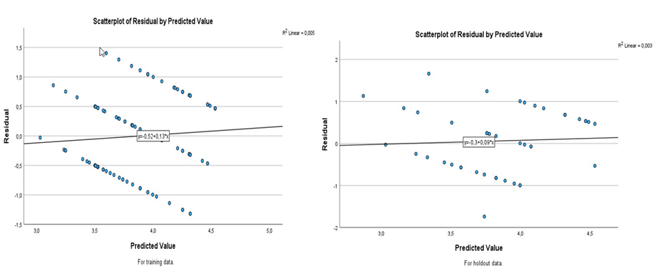
 Figure 4  - Scatterplot of residuals by predicted value for training and testing data.

As can be seen in Figure 4, there was a decrease in the slope of the regression line and the definition of the regression equation (holdout data). Analogously, average cross-validation is shown in Figure 5; MSE vs alpha (or λ) and R² vs alpha (or λ).

 

 

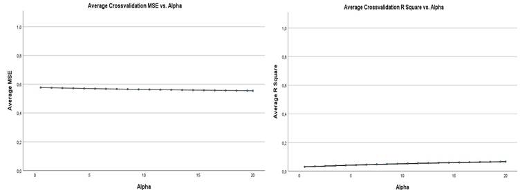
Figure 5 - cross-validation; MSE vs alpha (or λ) te R² vs alpha (or λ).

 

In parallel, L1 regularization (LASSO), cross-validation was performed on the same data; λ_max=20, λ_min=0.5, λ_interval=1. Cross-validation λ=1-20 with 5 iterations was performed on the total data set. The results indicate that the values ​​of all lambdas 1-20 for all categories of predictor variables, beta coefficients are zero (β_std=0; β=0);  β=0 which indicates the impossibility of interpreting the regression model (which is often the case with LASSO regression). In comparison with L1 regulation average MSE =0.60587 (λ1-λ20), and Average R² is unchanged (λ1-λ20).

The initial linear regression analysis was conducted using three predictor variables with ordinary least squares (OLS). After applying L2 regularization (Ridge regression) with cross-validation (λmax = 20, λmin = 0.5, λinterval = 1.0, using 5 folds, iterations), there was a notable reduction in the beta coefficients across the categories. This adjustment resulted in a decrease in mean squared error (MSE) and an increase in the R-squared (R²) value as the regularization parameter λ increased.

Initially, the OLS regression model was examined using a Bayesian approach, which favored the alternative hypothesis with a Bayes Factor of BF(10) = 17.938. The R² value was found to be 0.303, with an adjusted R² of 0.239. In contrast, the application of L1 regularization (LASSO) rendered the model uninterpretable due to insignificance, suggesting a type II error.

Conclusion

LASSO and RIDGE linear regressions offer improvements over ordinary least squares (OLS) regression, particularly in controlling overfitting and providing more reliable and accurate regression parameters. Their use is especially beneficial in situations with significant multicollinearity. One key difference between the two methods is that LASSO regression often reduces beta coefficients to nearly zero. While this can increase the risk of Type II errors, it can also result in better values for the coefficient of determination (R²).

Geraldo-Campos, Soria, and Pando-Ezcurra (2022) conducted a study comparing the predictive capabilities of four predictors on credit risk using a sample of 501298 companies in Peru. They found that LASSO regression (λ60 = 0.00038; RMSE = 0.357368) outperformed RIDGE regression in terms of predictive power. Wanishsakpong, Notodiputro, and Anwar (2024) examined the predictive roles of LASSO and RIDGE regressions in their analysis of daily temperatures in Taiwan. Their results showed that RIDGE regression successfully reduced the number of predictors from 32 to 13 and achieved better outcomes than LASSO regression in terms of MSE and R² values. Ren (2024) investigated the Student Performance Data Set and compared the predictive performance of LASSO, RIDGE, and ELASTIC NET regressions. The findings indicated that LASSO regression provided the best predictions for grades based on this dataset, while RIDGE regression performed the worst.

Overall, both L1 (LASSO) and L2 (RIDGE) regularizations effectively address issues of overfitting and multicollinearity, leading to more accurate and reliable regression parameters.

It is important to consider that both LASSO and RIDGE regression are iterative procedures, and their outcomes depend on several factors: the number of k-fold cross-validation, the number of k-iterations, the distribution of training and testing data, and the value of lambda (though this is a minor concern). As noted by Irandoukht (2021), both LASSO and RIDGE regression are subjective techniques, so caution should be exercised in their application and interpretation.

The findings of this study emphasize the need for caution when using LASSO regression in particular, as the model may become uninterpretable (resulting in beta zero coefficients), while results from Ordinary Least Squares (OLS) regression, RIDGE regression, and Bayesian inference (BS) suggest otherwise.

 

CONFLICTS OF INTEREST

There is no conflict of interest related to any aspect of this work.

ACKNOWLEDGMENTS

I would like to thank my colleague Irena for the matrix used for the empirical part and the reviewer's valuable suggestions. I am grateful to Fisher Library The University of Sydney for the space to work.

 

Literature

Dempster, A. P., Schatzoff, M., & Wermuth, N. (1977). A simulation study of alternatives to ordinary least squares. Journal of the American Statistical Association, 72, 77-91.

Geraldo-Campos, L., Soria, Alberto J., Pando-Ezcurra, T. (2022). Machine Learning for Credit Risk in the Reactive Peru Program: A Comparison of the Lasso and Ridge Regression Models. Economies, 10, 188. https://doi.org/10.3390/economies10080188

Hastie, T., Tibshirani, R., Friedman, J. (2009). The Elements of Statistical Learning Data Mining, Inference, and Prediction- second edition. Springer. http://dx.doi.org/10.1007/978-0-387-84858-7

Hoerl, Arthur E & . Kennard, Robert W. (1975). Ridge regression iterative estimation of the biasing parameter. Communications in Statistics - Theory and Methods, 5, 77-88.

Kennedy, E. (1988). Biased estimators in explanatory research: An empirical investigation of mean error properties of ridge regression. Journal of Experimental Education, 56, 135-141.

Irandoukht, A. (2021). Optimum Ridge Regression Parameter Using R-Squared of

Prediction as a Criterion for Regression Analysis. Journal of Statistical Theory and  

Applications, 20(2), 242–250.

Kampe, J.,  Brody, M., Friesenhahn, S., Garrett, A., Hegy, M. (2017). Lasso with Centralized Kernel. Final report - https://vadim.sdsu.edu/reu/2018-3.pdf Marquardt,

Marquardt, D. W., & Snee, R. D. (1975). Ridge Regression in Practice. The American Statistician, 29, 3-20.https://doi.org/10.1080/00031305.1975.10479105

Nelson, M., Biu, O. E., & Onu, O. H. (2024). Multi-Ridge, and Inverse- Ridge Regressions for Data with or Without Multi-Collinearity for Certain Shrinkage Factors. International Journal of Applied Science and Mathematical Theory, 10(2), 29-41.

Ren, P. (2024). Comparison and analysis of the accuracy of Lasso regression, Ridge regression and Elastic Net regression models in predicting students' teaching quality achievement. Applied and Computational Engineering, 51(1),313-319

DOI: 10.54254/2755-2721/51/20241625

Tibshirani, R. (1996). Regression Shrinkage and Selection via the Lasso. Journal of the Royal Statistical Society. Series B (Methodological), 58(1), 267-288.

Van del Velde, F., Piersoul, J., De Smet, I., Rupper, E. (2021). Changing Preferences in Cultural References. In; Kristiansen, G.,  Franco, K., ‎De Pascale, S.(Eds). Cognitive Sociolinguistics Revisited (584-595). Berlin/Boston; Walter de Gruyter.

Walker, David A. (2004). Ridge Regression as an Alternative to Ordinary Least Squares: Improving Prediction Accuracy and the Interpretation of Beta Weights. AIR Professional File, Number 92.

Wanishsakpong, A., Notodiputro, K. Anwar (2024). Comparing the performance of Ridge Regression and Lasso techniques for modeling daily maximum temperatures in the Utraradit Province of Thailand. Modeling Earth Systems and Environment,10, 5703–5716.   https://doi.org/10.1007/s40808-024-02087-z

Wessel, N. van Wieringen (2023). Lecture notes on ridge regression. This document is distributed under the Creative Commons Attribution-Non Commercial-ShareAlike license: http://creativecommons.org/licenses/by-nc-sa/4.0/ (accessed 4.11.2024)