
Misconceptions of the p-value - let us use new approaches and procedures
Siniša Opić, Majda RijavecUniversity of Zagreb, Faculty of Teacher Education |
|
Pedagogy, didactics and inclusion in education |
Number of the paper: 21 |
Original scientific paper |
Abstract |
|
Back in 1925, in the book Statistical Methods for Research Workers, Ronald Fisher defined the statistical significance p<0.05, and today almost a hundred years later, there is a growing need to redefine this arbitrary and often misinterpreted value indicating existence/nonexistence of differences, correlations or effects. P-value indicates that the null hypothesis is true, i.e. the probability that the result was accidental, but it is not related to whether the alternative hypothesis is true or false. Also, the p-value depends on sample size. The larger the sample, the smaller the associated p-value and the higher the risk of “accidental” significance at the 5% threshold. Therefore, in certain cases, it is suggested to use Bayesian statistics whose parameters are more informative rather than the commonly used statistical significance (p <0.05). On the basis of various simulations, this paper proposes a tripartite standard statistical inference approach which include Confidence Intervals (CI), effect size, and Bayesian procedure. The p-value should be one of the inference approaches, but not necessarily the only one. The dichotomous (yes/no) approach based on the rejection or confirmation of a hypothesis should be replaced by a polystochastic one. |
|
Key words |
|
Bayesian inference; confidence intervals; effect size; p-value; statistical significance |
Introduction
In March 2019, in the journal Nature 854 authors (signatories) published an article titled “Retire statistical significance” as an appeal for eliminating the binary statistical significance decision. Statistical significance (p-value) is treated as a boundary between good and evil, truth and lie, and as a solution to this pervasive and ubiquitous problem signatories require other statistical approaches and thresholds (Amrheim et al., 2019). In this paper, we will address the history of introducing p-value, its limitations, and suggestions for overcoming them.
History
At the beginning of the last century, Karl Pearson was the first who formally introduced the p-value in his Pearson's chi-squared test, using the chi-squared distribution and notating it with capital P (Pearson, 1900). However, it was Ronald Fisher (Fisher, 1925) who later developed the theory behind the p-value and first provided the means to calculate the p-value in a great number of situations. This theory, together with the theory of Neyman and Pearson (1933), provided researchers with important quantitative tools to confirm or reject their hypotheses. In this paper we will consider the application of p-values based on Fisher’s, Nayman-Pearson’-s, and Bayesian schools of statistical inference.
Simply put, Fisher claimed that a p-value is a measure of the probability that an observed difference or association could have occurred just by random chance. The smaller the p-value, the stronger the evidence against the null hypothesis of no difference or association. Fisher did not intend to use the p-value as a decision-making instrument but to “provide researchers with a flexible measure of statistical inference within the complex process of scientific inference” (Kyriacou, 2016).
Later, Neyman and Pearson (1933) formalized the hypothesis testing process setting a prior value for the rejection of the null hypothesis known as the significance level. This p-value was usually, by convention, selected to be below .05. A p-value below .05 is conclusively determined to be “statistically significant,” leading to the rejection of the null hypothesis. Contrary to that, if the p-value is above .05 the null hypothesis is not rejected and is assumed to be true. Actually, the p-value presents how incompatible our data are with a null hypothesis, but does not present at all how incompatible our data are with an alternative hypothesis. This fact frequently causes misleadings in inferential statistics.
This process can lead to two potential errors. The first is rejecting the null hypothesis when it is actually true. This is known as a type I error and will occur with a frequency based on the level selected for determining significance (α). If α is selected to be .05, then a type I error will occur 5% of the time. The second potential error is accepting the null hypothesis when it is actually false. This is known as type II error. The complement of a type II error is to reject the null hypothesis when it is truly false.
Limitations of P-value
Reporting p-values is common in scientific publications (Cristea & Ioannidis, 2018). However, nowadays it is widely recognized that p-value is very often and very easily misinterpreted.
Firstly, the problem related to p-value is its use in an all-or-nothing fashion to decide about a statistical hypothesis (i.e., Masson, 2011; Stern, 2016). Once the researcher finds the p-valued to be under the threshold of 0.05 the typical conclusion is that the null hypothesis is unlikely to be true, rejects the null hypothesis, and accepts the alternative hypothesis instead. However, it is often forgotten that the p-value is predicated on the null hypothesis being true, but it is not related to whether the alternative hypothesis is true or false. If the p-value is less than .05 the null hypothesis can be rejected. But this does not mean that there is a 95% probability that the alternative hypothesis is true (Cohen, 1994). The second problem lies in a common mistake that rejecting the null hypothesis doesn’t mean there is no effect in experimental design. In an analysis of 406 articles, almost half of them are wrongly interpreted; nonsignificant values are interpreted as there is no effect (Schatz et al., 2005). Further, the simple distinction between "significant" and "non-significant" is not very reliable. For example, there is little difference between the evidence for p-values of 0.04 and of 0.06. Rosnow and Rosenthal (1989) state: “surely, God loves the .06 nearly as much as the .05” (p. 1277).
Secondly, a p-value depends on the sample size. The larger the sample, the smaller the associated p-value and the higher the risk of “accidental” significance at the 5% threshold (Cohen, 1990). Inevitably, with a big enough sample size, the null hypothesis will be rejected.
Obviously, interpreting only a p-value is not a good approach in inferential statistics. Dunleavy and Jeffrey (2021) also note this point in stipulating the three basic Dominant Statistical Inference Schools: School Frequentist, Bayesian, and Likelihood. Within the frequentist approach, we ask What should we do? and use p-values, confidence, a, b, power, Type I error, and Type II error. The Bayesian approach deals with the question What should I believe? and use Bayes factors, credible intervals, prior and posterior probability. Finally, within the likelihood approach, we ask What does the evidence say? and apply likelihood ratios, likelihood intervals, the likelihood principle, and the law of likelihood.
What can be used instead of the p-value?
Despite the fact that many authors pointed to the common misconceptions about p-values for more than half a century (e.g., Bakan, 1966; Rozeboom, 1960) there is still a strong over-reliance on p-values in the scientific literature.
Due to the limitations of p-values, it has been recommended to replace (Cumming, 2014) or supplement (Wasserstein & Lazar, 2016) p-values with alternative statistics, such as confidence intervals, effect sizes, and Bayesian methods.
Confidence intervals
As mentioned above, interpretation of results based only on p-values can be misleading. Furthermore, effect may not be meaningful in the real world since it might be too small to be of any practical value.
Generally, the confidence interval is more informative than statistical significance since it provides information about statistical significance, as well as the direction and strength of the effect (Shakespeare et al., 2001). For example, if the level of confidence is 95 % it means we are 95 % confident that the interval contains the population means. CI 95% indicates that 95 out of 100 times the range of values contains the true population mean as estimated from the sample (Anderson, 1998). Potter (1994) indicates the importance of confidence level in case our data does not result in finding the statistically significant difference or effect. This is very important particularly when our data are of near-borderline significance, e.g. p = 0.06.
Although CI is more informative than p-value, it does so with moderate precision at the expense of larger sample size (Liu, 2013). Although sample size has a negative effect on the level of statistical significance, i.e. on large samples it increases the probability of confirming statistical significance, these large samples have a positive effect on CI because it reduces their interval. That is why CI with large width is not so informative. Thus, according to Cohen (1994) the width of the confidence interval ‘‘provides us with the analog of power analysis in significant testing—larger sample sizes reduce the size of confidence intervals as they increase the statistical power’’ (p. 1002).
It should be noted that although CI seems easier to interpret than statistical significance, both cause many misunderstandings in science so there is a need for better statistical training in science. Lyu et al. (2020) conducted a research in China which included 1479 researchers and students in different fields of research.. The results revealed that for significant (i.e., p < .05, CI does not include zero) and non-significant (i.e., p > .05, CI includes zero) conditions, most respondents, regardless of academic degrees, research fields and stages of career, could not interpret p-values and CIs accurately. Moreover, the majority were confident about their (inaccurate) judgments.
Describing differences between CI and statistical significance, du Prel et al. (2009) clarified that statistical significance and confidence interval (CI) are not contradictory statistical concepts, they are complementary. Additionally, confidence intervals ensure information about statistical significance, such as direction and strength of the effect (Shakespeare et al., 2001). Since p-value and confidence interval provide complementary information about the statistical probability and conclusions regarding the significance of study findings, both measures should be reported.
The Effect Size
Although a p-value can indicate differences between conditions, it cannot answer a very relevant question about how large this difference is. This question can be answered by calculating the “effect size”, which quantifies differences. In other words, effect size is the magnitude of the difference between groups. Thus, in reporting results, both p-values and effect size should be reported.
Why is reporting only a significant p-value not enough? As already mentioned, with a sufficiently large sample, a statistical test will almost always demonstrate a significant difference. However, although significant, very small differences are often meaningless. Unlike p-value, the effect size is independent of sample size.
The adequate effect size for the comparison between two or several means is Cohen's d, used with reporting t-test and ANOVA results. Effect size is calculated by dividing the difference between the two groups by the standard deviation of one of the groups. Cohen classified effect sizes as small (d = 0.2), medium (d = 0.5), and large (d ≥ 0.8). Cohen d shows the real difference of arithmetic means regardless of the measurement scale. It allows the comparison of real, practical differences in different studies and is also suitable for meta-analyses. Glass’s delta is a version of Cohen's effect size and is suitable for experimental designs. It represents the ratio of the uncorrected difference of the arithmetic means of the two groups and the standard deviation of the control group. It is necessary to know the standard deviation of the control group (d). In the case of small samples and disproportion of the subsamples which are compared, Hedge`s g (Δ is a good solution.
Bayes factor
One of the proposed alternatives to p-value is to use Bayesian inference. Bayesian statistics combines observed data with prior information about phenomena in order to make inferences by using Bayes’ theorem. Bayes’ theorem updates prior to the posterior distribution. The concept of Bayesian is updating probabilities in case of new evidence. The concept of Bayesian inference (Bayes’ theorem) is shown in Figure 1.
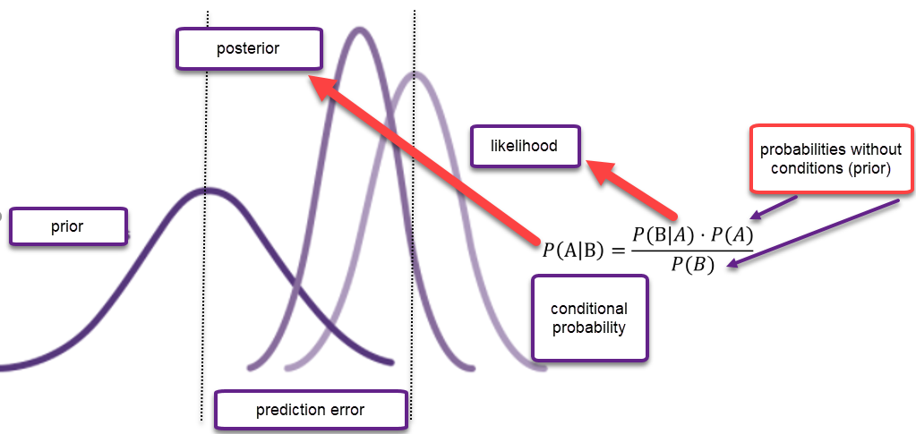
Figure 1. Bayes` theorem
A considerable number of researchers paid attention to Bayes’ factor as an alternative to classical procedure (Hoijtink, van Kooten, & Hulsker, 2016; Jarosz & Wiley, 2014; Morey & Rouder, 2011; Stern, 2016).
As already mentioned, the p-value provides information only about the probability that the null hypothesis is true. Contrary to that, Bayesian framework allows us to quantify how much more likely the data are under the null hypothesis (H0) compared to the alternative hypothesis (H1), given a prior probability. The Bayes factor (BF) a popular implementation of Bayesian hypothesis testing, directly addresses both the null and the alternative hypotheses and quantifies the degree to which the data favor one of two hypotheses by considering the prior odds (Held & Ott, 2018). When BF equals one, data provide the same evidence for both hypotheses. However, when BF is higher than one, the null hypothesis is more probable than the alternative one. For example, if we observed that BF 01 = 5, we could conclude that the null hypothesis is five times more likely than the alternative (Ruiz-Ruano & Puga, 2018).
Bayes factor between 1 and 3 indicates anecdotal evidence for H0, between 3 and 10 indicates substantial evidence for H0. On the other hand, 1/3 and 1 indicate anecdotal evidence for H1, and between 1/10 and 1/3 indicates substantial evidence for H1 (George Assaf & Tsionas, 2018).
The correct use of p-values and Bayesian methods will often lead to similar statistical inferences.
Research example
Small sample, larger sample and p-value
We tested differences between three groups of students, undergraduate (n=71), graduate (n=78) and integrated undergraduate and graduate (n=63) on the dependent variable -quality of on-line classes.
First, we performed One-way ANOVA analysis on a smaller sample of 50% randomly selected cases. The results showed no significant difference between samples [F(2. 119) = 1.747; p = 0.179; η2 =0.03]. So, Ho was accepted and it was concluded that the three groups of students do not differ in their assessments of the quality of on-line classes, i.e. they belong to the same population.
In the next analysis the whole sample was used. The results of the One-way ANOVA rejected Ho [F(2. 209) = .331. p = 0.038]. This means that those subsamples of students do not belong to the same population, i.e. there is a difference between them with respect to the quality of on-line classes. However, is this for real?
Effect size, Eta square (η2 =0.031) indicates the low real difference between subsamples on the dependent variable. So, although we rejected Ho (p=0.038) and accepted that significant differences exist between the three groups, these differences are small and reflect no real/practical differences between subsamples (Table 1).
Table 1. ANOVA analyses for smaller and larger sample
|
|
undergraduates |
graduates |
integrated |
|
|
|||
|
|
M |
SD CI |
M |
SD CI |
M |
SD CI |
p |
η2 |
|
smaller sample (N=110) |
3.63 |
1.19 3.22-4.04 |
3.83 |
.92 3.54-4.12 |
4.06 |
.69 3.82-4.30 |
.179 |
0.032 |
|
larger sample (N=212) |
3.54 |
1.17 3.26-3.81 |
3.81 |
.91 3.60-4.01 |
3.97 |
.84 3.76-4.18 |
.038 |
0.038 |
When half of the sample was used (N=110), the results indicated that the p-value was ,179 so the H0 was accepted suggesting no difference between samples. Furthermore, the confidence intervals overlapped, the fact that is usually the indication of no difference between samples.
However, when the whole sample was used the p-value was ,038 thus the H0 was rejected suggesting significant difference between samples. So, if we use only p-value as indicator of significant difference we will conclude that these three samples are significantly different in overall assessment of the quality of on-line classes. However, upon inspection of Table 1, it is evident that the confidence intervals in this sample also overlapped, and effect size, Eta square d was almost the same as in the first sample. These indicators, contrary to p-value, point to no meaningful, real difference between the samples.
It is easy to see that adding more participants to the sample led to the smaller associated p-value and rejection of H0, while the other two indicators (CI and effect size) did not change. Thus, using only p-value as indication of difference can prompt some researchers to enlarge the samples in other to “fish” for significant difference and to neglecting other indicators in this process.
In order to further inspect the data we performed Bayesian ANOVA analysis. The Bayesian results are shown in Table 2.
|
Table 2. ANOVA with Bayes Factor |
||||||
|
Dependent variable |
Sum of Squares |
df |
Mean Square |
F |
Sig. |
Bayes Factora |
|
Between Groups |
6.494 |
2 |
3.247 |
3.331 |
.038 |
.122 |
|
Within Groups |
203.714 |
209 |
.975 |
|
|
|
|
Total |
210.208 |
211 |
|
|
|
|
|
|
||||||
Bayes Factor (Bf=1.22) indicates almost no evidence for either null or alternative hypothesis. BF about value 1 puts us in a tentative situation because in this case there is no evidence for H1. Furthermore, it is informative to see posterior mean and Confidence interval (95%CI) presented in Table 3.
|
Table 3. Bayesian Estimates of Coefficients |
|||||
|
Parameter |
Posterior |
95% Credible Interval |
|||
|
Mode |
Mean |
Variance |
Lower Bound |
Upper Bound |
|
|
undergraduate |
3.535 |
3.535 |
.014 |
3.304 |
3.766 |
|
graduate |
3.808 |
3.808 |
.013 |
3.587 |
4.028 |
|
integrated undergraduate and graduate |
3.968 |
3.968 |
.016 |
3.723 |
4.213 |
|
|
|||||
|
If we compare prior means (µ1=3.54; µ2=3.81; µ3=3.97) with posterior there is almost no difference. Additionally, 95% CI of prior means; µ1 (LB=3.26; UB=3.81); µ2(LB=3.60; UB=4.01); µ3 (LB=3.76; UB=4.18) are just slightly different from posterior CI (Table 3). CI of mean is very informative because it indicates that we are 95% sure that the population mean lies in this range. Ranges of CI (lower and upper) are slightly (smaller) which indicates more precise value of the mean. A posterior, log likelihood and prior distribution are shown in Figures 2,3 and 4. |
|||||
|
|
|||||
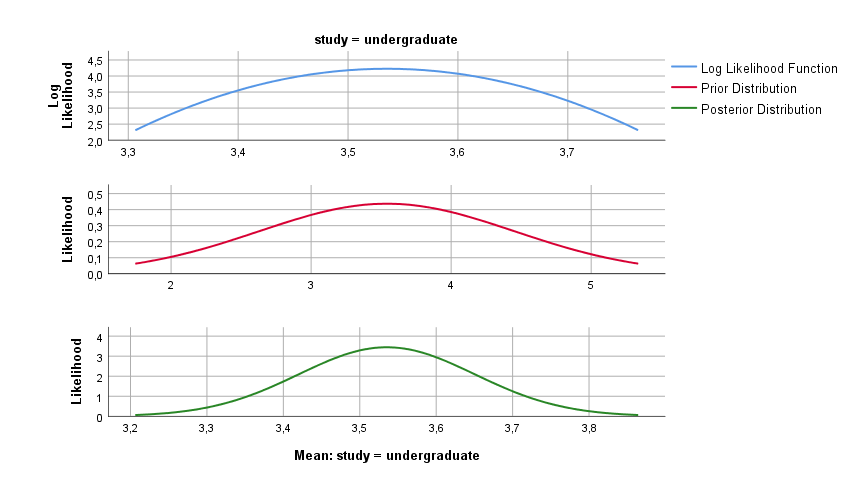
Figure 2. Posterior log likelihood and prior distribution of undergraduate study (sample 1)

Figure 3. Posterior, log likelihood and prior distribution of graduate study (sample 2)

Figure 4. Posterior, log likelihood and prior distribution of graduate study (sample 3)
A posterior distribution is an updated prior distribution with new evidence (data), or inverse conditional probability of the likelihood. When the prior and posterior distributions are similar (same family) this indicates that the model/hypothesis is well set, i.e. even after supplementing/updating the prior distribution with “new evidence” there was no large deviation in the posterior distribution (conditional probability) compared to the prior distribution. The differences between the posterior and prior distributions are relative to the Bayesian values. If a posterior probability (also distribution) is similar to some adjustment on prior probability, it means that the less confirmed adjustment determines better prior model.
Conclusion
Keeping in mind all of the abovementioned limitations, obviously there is a need to redefine the use of the p-value. We believe that the solution is not to completely abolish the p-value, but to extend statistical inference to the statistical areas described in the paper. We propose a tripartite standard statistical inference approach: Statistical significance (CI), effect size, and Bayesian procedure. The p-value should be one of the inference approaches, but not the only one. The dichotomous approach based on the rejection or confirmation of a hypothesis (yes/no) should be replaced by a polystochastic one.
References
Anderson, H. G., Kendrach, M. G., & Trice, S. (1998). Understanding statistical and clinical significance: hypothesis testing. Journal of Pharmacy Practice, 11(3), 181–195. doi:10.1177/089719009801100309
Amrheim, V. et al. (2019). Retire Statistical Significance. Nature, 567(7748), 305–307.
Bakan, D. (1966). The test of significance in psychological research. Psychological Bulletin, 66, 423–437. doi:10.1037/h0020412
Cohen, J. (1990). Things I have learned (so far). American Psychologist, 45, 1304. doi:10.1037/0003-066X.45.12.1304
Cohen, J. (1994). The Earth is round. American Psychologist, 49, 997–1003. doi:10.1037/0003-066X.49.12.997
Cramer, D. i Howitt, D. L. (2004). The SAGE Dictionary of Statistics: A Practical Resource for Students in Social Sciences. London: SAGE Publications Ltd.
doi: 10.4135/9780857020123
Cristea, I. A. & Ioannidis, J.P.A. (2018). P values in display items are ubiquitous and almost invariably significant: A survey of top science journals. Plosone Collections, 13(5). doi: 10.1371/journal.pone.0197440
Cumming, G. (2014). The new statistics: Why and how. Psychological Science, 25, 7–29. doi:10.1177/0956797613504966
Du Prel, J. B., Hommel,G., Röhrig, G. B. & Blettner, M. (2009). Confidence Interval or P-Value?: Part 4 of a Series on Evaluation of Scientific Publications. Deutsches Ärzteblatt International, 106(19), 335–339. doi: 10.3238/arztebl.2009.0335
Dunleavy, D. J. & Lacasse, J. R. (2021). The Use and Misuse of Classical Statistics: A Primer for Social Workers. Research on Social Work Practice, 31(5), 438–453. doi: 10.1177/10497315211008247
Fisher, R. A. (1925). Statistical Methods for Research Workers. Edinburgh, UK: Oliver and Boyd.
George Assaf, A. & Tsionas, M. (2018). Bayes factors vs. P-values. Tourism Management, 67, 17–31. doi: 10.1016/j.tourman.2017.11.011
Greene, W. (2003). Econometric Analysis, 5th ed. New York: Prentice Hall.
Held, L. & Ott, M. (2018). On p-values and Bayes factors. Annual Review of Statistics and Its Application, 5, 393–419.
Hoijtink, H., van Kooten, P. & Hulsker, K. (2016). Why Bayesian psychologists should change the way they use the Bayes Factor. Multivariate Behavioral Research, 51, 2–10. doi: 10.1080/00273171.2014.969364
Jarosz, A. & Wiley, J. (2014). What are the odds? A practical guide to computing and reporting Bayes factors. Journal of Problem Solving, 7, 2–9. doi: 10.7771/1932-6246.1167
Kyriacou, N. (2016). The Enduring Evolution of the P Value. JAMA, 315(11), 1113–1115
Leamer, E. (1978). Specification Searches: Ad Hoc Inference with Nonex- perimental Data. New York: Wiley Mingfeng.
Lin, H. C., Lucas, Jr. & Shmueli, G. (2013). Research Commentary—Too Big to Fail: Large Samples and the p-Value Problem. Information Systems Research, 24(4), 906–917.
Liu, X. S. (2013). Comparing Sample Size Requirements for Significance Tests and Confidence Intervals. Counseling Outcome Research and Evaluation, 4(1), 3–12. doi:10.1o177/2150137812472194
Lyu X. K., Xu Y., Zhao X. F., Zuo X. N., & Hu C.-P. (2020). Beyond psychology: prevalence of p value and confidence interval misinterpretation across different fields. Journal of Pacific Rim Psychology, 14(6). doi: 10.1017/prp.2019.28
Masson, M. E. J. (2011). A tutorial on a practical Bayesian alternative to null-hypothesis significance testing. Behavioral Research, 43, 679–690. doi: 10.3758/s13428-010-0049-5
Morey, R. D. & Rouder, J. N. (2011). Bayes Factor approaches for testing interval null hypothesis. Psychological Methods, 16, 406–419. doi:10.1037/a0024377
Neyman, J. & Pearson, E. S. (1933). On the problems of the most efficient tests of statistical hypotheses. Philosophical Transactions of the Royal Society of London, 231A, 289–338. doi: 10.1098/rsta.1933.0009
Pearson K. (1900). On the criterion that a given system of deviations from the probable in the case of a correlated system of variables is such that it can be reasonably supposed to have arisen from random sampling. Philosophical Magazine, 5, 157–175.
Potter, R. H. (1994). Significance Level and Confidence Interval. Journal of Dental Research, 73(2), 494–496. doi:10.1177/00220345940730020101
Rosnow, R. L., & Rosenthal, R. (1989). Statistical procedures and the justification of knowledge in psychological science. American Psychologist, 44(10), 1276–1284. doi: 10.1037/0003-066X.44.10.1276
Rozeboom, W. W. (1960). The fallacy of the null-hypothesis significance test. Psychological Bulletin, 57, 416–428. doi:10.1037/h0042040
Ruiz-Ruano, A. M. & Puga, J. L. (2018). Deciding on Null Hypotheses using P-values or Bayesian alternatives: A simulation study. Psicothema, 30(1), 110–115. doi: 10.7334/psicothema2017.308
Schatz, P., Jay, K. A, McComb, J. i McLaughlin, J. R. (2005). Misuse of statistical tests in Archives of Clinical Neuropsychology publications. Archives of Clinical Neuropsychology. 20(8), 1053–9. doi: 10.1016/j.acn.2005.06.006.
Shakespeare, T. P., Gebski, V. J., Veness, M. J & Simes, J. (2001). Improving interpretation of clinical studies by use of confidence levels, clinical significance curves, and risk benefit contours. Lancet, 357, 1349–1353. doi: 10.1016/s0140-6736(00)04522-0
Stern, H. S. (2016). A test by any other name: P-values, Bayes Factors and statistical inference. Multivariate Behaviour Research, 51, 23–39. doi:10.1080/00273171.2015.1099032
Wasserstein, R. L., Schirm, A. L. & Lazar, N. A. (ur.). (2019). Statistical inference in the 21st century: A world beyond p < 0.05 [Special issue]. The American Statistician, 73(Suppl. 1). Dostupno na https://www.tandfonline.com/toc/utas20/73/sup1
|
|
2nd International Scientific and Art Faculty of Teacher Education University of Zagreb Conference Contemporary Themes in Education – CTE2 - in memoriam prof. emer. dr. sc. Milan Matijević, Zagreb, Croatia |

Zablude o p-vrijednosti – upotrijebimo nove pristupe i postupke |
Sažetak |
|
Davne 1925. godine u knjizi Statistical Methods for Research Workers, Ronald Fisher je definirao statističku značajnost p<0,05 i danas gotovo stotinu godina kasnije uočljiva je sve veća potreba redefiniranje te arbitrarno postavljene i vrlo često krivo interpretirana vrijednosti o postojanju/ nepostojanju razlika, povezanosti i učinaka. P-vrijednost ukazuje na to da je nul-hipoteza točna, tj. na vjerojatnost da je rezultat slučajno dobiven, ali ne odgovara na pitanja je li alternativna hipoteza točna ili netočna. Također, p-vrijednost ovisi o veličini uzorka. Što je uzorak veći to je p-vrijednost manja a time i je veći rizik “slučajne” značajnosti na razini od 5%. Na temelju različitih simulacija, u ovom radu se predlaže tripartitni standard statističkog zaključivanja koji uključuje intervale pouzdanosti (CI), veličinu učinka i bajezijansku proceduru. P-vrijednost može biti jedan od inferencijalnih pristupa, ali ne i jedini. Dihotomni (da/ne) pristup temeljen na prihvaćanju ili odbacivanju hipoteze treba zamijeniti polistohastičkim pristupom. |
|
Ključne riječi |
|
bajezijanska statistika; intervali pouzdanosti; veličina efekta; statistička značajnost |